Overview: In this assignment, we will work with historical national popular vote and state-level popular vote data from presidential elections. We will restructure the two data sets and eventually merge them, before running basic linear models to predict the national popular vote from the vote in certain states.

Data Details:

• File Name: state_2pv_1948_2020.csv

• These data contain the state-level popular vote from presidential elections from 1948 through 2020.

• File Name: nat_pv_1860_2020.csv

• These data contain the national-level popular vote from presidential elections from 1860 through 2020.

Question 1: Loading Packages and Data

Loading packages:

Once you install R and R Studio, you can open R Studio, which uses R in the background. The first thing to do within RStudio is to install and load the packages you will be using. You can read about packages and how to install them on Modern Dive Section 1.3. You will need two packages for this problem set: \texttt{tidyverse} and \texttt{ggplot2}. \footnote{One of the reasons R is such a widely used language is that there is a whole community that develops packages, which add functionality to the language. You can think of a package as just a collection of useful functions that aren’t available in base R.}

The instructions at that link are primarily for the point-and-click method of installing packages, but it’s also important to know how to do it via the command line. Some may find it easier as well. To install packages via the command line, simply run install.packages("package_name") in RStudio, making sure the package name is in quotes. Note that there are multiple ways to run a command within RStudio: one way is to type the command in the “Console” pane of RStudio and press Return/Enter on your keyboard. Another is to open a .Rmd file, create a code chunk, and press the green play button in its top-right corner.

Once you install the packages, you can run library(package_name) to load it into RStudio. Note that the package doesn’t need to be in quotes inside the library() function, but it can be if you like.

Load the packages ggplot2 and tidyverse in the code below.

library("ggplot2")
library("tidyverse")

## ── Attaching core tidyverse packages ──────────────────────── tidyverse 2.0.0 ──
## ✔ dplyr     1.1.4     ✔ readr     2.1.5
## ✔ forcats   1.0.0     ✔ stringr   1.5.1
## ✔ lubridate 1.9.3     ✔ tibble    3.2.1
## ✔ purrr     1.0.2     ✔ tidyr     1.3.1
## ── Conflicts ────────────────────────────────────────── tidyverse_conflicts() ──
## ✖ dplyr::filter() masks stats::filter()
## ✖ dplyr::lag()    masks stats::lag()
## ℹ Use the conflicted package (<http://conflicted.r-lib.org/>) to force all conflicts to become errors

Loading data:

After loading the packages we need, it’s time to read the data into R. But there’s one last step! Before you try to read data, it is a good idea to tell R where on your computer you’re working. To do that, you need to set your working directory. Remember, “directory” is just a computer science term for a folder on your computer. By setting your working directory, you’re telling R the folder in which to look for files. Usually it’s best practice to set your working directory to the directory that your code is in. To do that, just go to the toolbar at the top of your screen, select “Session”, hover over “Set Working Directory”, and select “To Source File Location”.

You can check your current working directory by running getwd() with nothing in the parentheses. Try running getwd() in the console to make sure your current working directory is the one where you have this file saved. Make sure that you have downloaded the data for this assignment into that same directory for the code below to work. This works because by setting the working directory you told R the folder where it will find the data.

Note: If you set the correct working directory but still get an error running the code below, you may also need to click the downward arrow next to the “Knit” button on the top of the “Source” pane and set Knit Directory to either Document Directory or Current Working Directory.

Load the data in the code chunk below:

nat <- read_csv("/Users/ellatrembanis/Desktop/Gov 1347/election-blog/election-blog/Week1/nat_pv_1860_2020.csv")

## Rows: 41 Columns: 3
## ── Column specification ────────────────────────────────────────────────────────
## Delimiter: ","
## dbl (3): year, npv_democrat, npv_republican
## 
## ℹ Use `spec()` to retrieve the full column specification for this data.
## ℹ Specify the column types or set `show_col_types = FALSE` to quiet this message.

state <- read_csv("/Users/ellatrembanis/Desktop/Gov 1347/election-blog/election-blog/Week1/state_2pv_1948_2020.csv")

## Rows: 1918 Columns: 10
## ── Column specification ────────────────────────────────────────────────────────
## Delimiter: ","
## chr (3): state, candidate, party
## dbl (7): year, state_fips, candidatevotes, totalvotes, vote_share, two_party...
## 
## ℹ Use `spec()` to retrieve the full column specification for this data.
## ℹ Specify the column types or set `show_col_types = FALSE` to quiet this message.

Question 2: Transforming Data in the Tidyverse

In this question, we will walk through a number of useful functions for wrangling data in tidyverse: select, arrange, mutate, filter, and group_by/summarize. You are not by any means required to use tidyverse in this course — feel free to use base R if you are more comfortable with it. But tidyverse has several data-wrangling tools that are often more efficient and intuitive than base R.

(a) Select

The select function is used when we want to focus on only certain variables (i.e., columns) in our data set. There may be many substantive reasons why we might want to remove certain columns, though sometimes we may just want to remove columns to reduce clutter in the data set. For the analysis we are conducting in this assignment, we do not need the vote totals — only two party vote share. Use the select function to limit the state-level data set to only the variables year, state, party and two_party_vote_share. Call this smaller dataframe state_select. Check the dimensions of the dataframe using the dim function: it should have four columns and 1918 rows.

state_select <- state |>
  select(year, state, party, two_party_vote_share)
dim(state_select)

## [1] 1918    4

(b) Arrange

The arrange function can be used to order the data set according to a given variable. Right now, the state_select dataframe is in alphabetical order by state. Suppose that we want to display the data set in order from most to least recent election. Use the arrange function to order the data set by year. Use the head function to ensure that elections from 2020 are indeed at the top of the data set.

Hint: Consider wrapping the year variable in the desc() function

state_select <- state_select |>
  arrange(desc(year))
head(state_select)

## # A tibble: 6 × 4
##    year state   party      two_party_vote_share
##   <dbl> <chr>   <chr>                     <dbl>
## 1  2020 Alabama Democrat                   37.1
## 2  2020 Alabama Republican                 62.9
## 3  2020 Alaska  Democrat                   44.7
## 4  2020 Alaska  Republican                 55.3
## 5  2020 Arizona Democrat                   50.2
## 6  2020 Arizona Republican                 49.8

(c) Mutate

The mutate function allows you to define new variables or redefine existing variables. Currently, the national data set only includes the overall vote share of the parties (e.g., Democratic votes divided by total votes). To be consistent with the state-level data, define new variables dem_tpv and rep_tpv as the two party vote share (as percentages) received by the Democratic and Republican candidates, respectively. Then select only the year, dem_tpv, and rep_tpv columns and save this dataframe as object national_mutate.

Hint: the Democratic two party vote share is equal to Democratic two party vote share divided by the Democratic two party vote share plus the Republican two party vote share. You should multiply by 100 to get vote shares as percentages.

national_mutate <- nat |>
  mutate(
    dem_tpv = 100*npv_democrat/(npv_democrat + npv_republican),
    rep_tpv = 100*npv_republican/(npv_democrat + npv_republican)
  ) |>
  select(year, dem_tpv, rep_tpv)
head(national_mutate)

## # A tibble: 6 × 3
##    year dem_tpv rep_tpv
##   <dbl>   <dbl>   <dbl>
## 1  2020    52.2    47.8
## 2  2016    51.1    48.9
## 3  2012    52.0    48.0
## 4  2008    53.7    46.3
## 5  2004    48.8    51.2
## 6  2000    50.3    49.7

(d) Filter

While the select function allows you to focus on certain columns in a dataframe, the filter function allows you to focus on certain rows. The state-level data set only includes data going back to 1948, whereas the national data dates to 1860. Since we plan to merge these data sets, use the filter function to subset your mutated national data to only elections after 1948 (including 1948 itself). Save this dataframe as national_mutate_filter.

national_mutate_filter <- national_mutate |>
  filter(year >= 1948)

(e) Group_by and Summarize

The group_by and summarize functions are great for quickly producing key summary information about your dataset. Suppose we want to compare the average Democratic two party vote share in 21st century elections between California and Massachusetts (note: consider the 2000 election as part of the 21st century). Which state, in recent years, has been more Democratic? Use the filter function to subset the data set to 21st century elections and subset the data to only consider the Democratic vote share. Then, use group_by and summarize to get the average two party vote share by state. Finally, use the filter function again to subset the summarized data set to only California and Massachusetts.

state_select |>
  filter(year >= 2000) |>
  filter(party == "Democrat") |>
  group_by(state) |>
  summarize(
    avg_dem_share = mean(two_party_vote_share, na.rm = T)
  ) |>
  filter(state == "California" | state == "Massachusetts")

## # A tibble: 2 × 2
##   state         avg_dem_share
##   <chr>                 <dbl>
## 1 California             61.1
## 2 Massachusetts          64.0

Massachusetts has been more Democratic, on average, in 21st-century presidential elections.

Question 3: Pivoting Data: Wide to Long

We’re nearly ready to merge the national- and state-level data into a single data frame. However, you may notice that the two data-frames treat party differently. In the national data set, there are two separate columns for two party vote (dem_tpv and rep_tpv). This data structure is known as ‘‘wide’’ because there are relatively more columns and fewer rows. The state-level data, on the other hand, has a single column for two party vote and a separate column (party) indicating whether the candidate is a Republican or Democrat. This data structure is ‘’long’’ because there are relatively more rows and fewer columns. Use the pivot_longer function to convert the wide national data into the long format, and call this new dataframe national_mutate_filter_long.

Hint: After pivoting, this new dataframe should have three columns: the year, the party, and the national two party vote share (call this column national_two_party_vote_share or similar). To make things consistent with the state-level data, use the mutate function to make the party variable contain entries of either ‘‘Democrat’’ or ‘‘Republican.’’

national_mutate_filter_long <- national_mutate_filter |>
  pivot_longer(
    cols = c(dem_tpv, rep_tpv),
    names_to = "party",
    values_to = "national_two_party_vote_share"
  ) |>
  mutate(
    party = ifelse(party == "dem_tpv", "Democrat", "Republican")
  )
head(national_mutate_filter_long)

## # A tibble: 6 × 3
##    year party      national_two_party_vote_share
##   <dbl> <chr>                              <dbl>
## 1  2020 Democrat                            52.2
## 2  2020 Republican                          47.8
## 3  2016 Democrat                            51.1
## 4  2016 Republican                          48.9
## 5  2012 Democrat                            52.0
## 6  2012 Republican                          48.0

Question 4: Merging Data Sets: Full_Join

Finally, we’re ready to merge the national_mutate_filter_long and state_select dataframes. Use the full_join function to merge the two dataframes by year and party.

Call this merged data set combined_data. It should contain 5 columns: the state, party, year, two party vote share in the state, and two party vote share for the candidate nationally.

Note that you could also use the right_join, left_join, or inner_join here. In general, it is usually safest to start with full_join so that you don’t inadvertently eliminate rows in the data set. Suppose for example you are trying to merge data sets by congressional district. If North Dakota’s lone district is called ND-01 in one dataframe and ND-AL in the other, neither will be included in the joined dataframe if you use inner_join.

combined_data <- national_mutate_filter_long |>
  full_join(state_select, by = c("year", "party"))
head(combined_data)

## # A tibble: 6 × 5
##    year party    national_two_party_vote_share state      two_party_vote_share
##   <dbl> <chr>                            <dbl> <chr>                     <dbl>
## 1  2020 Democrat                          52.2 Alabama                    37.1
## 2  2020 Democrat                          52.2 Alaska                     44.7
## 3  2020 Democrat                          52.2 Arizona                    50.2
## 4  2020 Democrat                          52.2 Arkansas                   35.8
## 5  2020 Democrat                          52.2 California                 64.9
## 6  2020 Democrat                          52.2 Colorado                   56.9

Question 5: Pivoting Data: Long to Wide

In the previous two questions, we pivoted the national data to a long format and then merged the two data sets. Now, let’s merge the data sets in the wide format. Start with the state_select dataframe and use the pivot_wider function so that that each column represents the vote share for a given party in a specific state. Call this dataframe combined_data_wide.

Merge this with the national_mutate_filter dataframe so that you also have one column representing the national Democratic two party vote proportion and one column representing the national Republican two party vote proportion.

Hint: You should end up with 19 rows, one for each election year. You should have 105 columns: the year, the national Democratic vote share, the national Republican vote share, and the Democratic and Republican vote shares in each of the 50 states + DC

combined_data_wide <- state_select |>
  pivot_wider(
    names_from = c("party", "state"), values_from = c(two_party_vote_share)
  ) |>
  full_join(national_mutate_filter, by = "year")
head(combined_data_wide)

## # A tibble: 6 × 105
##    year Democrat_Alabama Republican_Alabama Democrat_Alaska Republican_Alaska
##   <dbl>            <dbl>              <dbl>           <dbl>             <dbl>
## 1  2020             37.1               62.9            44.7              55.3
## 2  2016             35.6               64.4            41.6              58.4
## 3  2012             38.8               61.2            42.7              57.3
## 4  2008             39.1               60.9            38.9              61.1
## 5  2004             37.1               62.9            36.8              63.2
## 6  2000             42.4               57.6            32.1              67.9
## # ℹ 100 more variables: Democrat_Arizona <dbl>, Republican_Arizona <dbl>,
## #   Democrat_Arkansas <dbl>, Republican_Arkansas <dbl>,
## #   Democrat_California <dbl>, Republican_California <dbl>,
## #   Democrat_Colorado <dbl>, Republican_Colorado <dbl>,
## #   Democrat_Connecticut <dbl>, Republican_Connecticut <dbl>,
## #   Democrat_Delaware <dbl>, Republican_Delaware <dbl>,
## #   `Democrat_District Of Columbia` <dbl>, …

Question 6: Running Some Very Basic Linear Models

(a) Simple Regression

With the wide combined data set, run a basic linear model using the lm function to predict the national two-party Democratic vote share from the two party Democratic vote share in Florida. Interpret the model coefficients and use the summary function to determine whether the relationship is statistically significant.

lm1 <- lm(dem_tpv ~ Democrat_Florida, data = combined_data_wide)
summary(lm1)

## 
## Call:
## lm(formula = dem_tpv ~ Democrat_Florida, data = combined_data_wide)
## 
## Residuals:
##     Min      1Q  Median      3Q     Max 
## -4.9092 -1.2060 -0.0151  1.4236  9.1158 
## 
## Coefficients:
##                  Estimate Std. Error t value Pr(>|t|)    
## (Intercept)       20.4329     4.9123   4.160 0.000657 ***
## Democrat_Florida   0.6217     0.1044   5.953 1.57e-05 ***
## ---
## Signif. codes:  0 '***' 0.001 '**' 0.01 '*' 0.05 '.' 0.1 ' ' 1
## 
## Residual standard error: 3.208 on 17 degrees of freedom
## Multiple R-squared:  0.6758,	Adjusted R-squared:  0.6568 
## F-statistic: 35.44 on 1 and 17 DF,  p-value: 1.572e-05

Interpretation: The coefficient of 0.6217 means that for every one percentage point increase in Democratic vote share in Florida, we would expect the candidate to gain 0.6217 percentage points nationally. This relationship is statistically significant, with a test statistic approaching 6.

(b) Multiple Regression

Now run a model predicting the national two-party Democratic vote share from the two party Democratic vote share in Florida and New York. What do you notice about the magnitude of the coefficient on the Florida term relative to part (a)?

lm2 <- lm(dem_tpv ~ Democrat_Florida + `Democrat_New York`, 
           data = combined_data_wide)
summary(lm2)

## 
## Call:
## lm(formula = dem_tpv ~ Democrat_Florida + `Democrat_New York`, 
##     data = combined_data_wide)
## 
## Residuals:
##     Min      1Q  Median      3Q     Max 
## -2.8756 -1.0588 -0.1154  0.5401  6.1314 
## 
## Coefficients:
##                     Estimate Std. Error t value Pr(>|t|)    
## (Intercept)         13.73627    3.51341   3.910 0.001248 ** 
## Democrat_Florida     0.37573    0.08544   4.398 0.000449 ***
## `Democrat_New York`  0.32424    0.06710   4.833 0.000184 ***
## ---
## Signif. codes:  0 '***' 0.001 '**' 0.01 '*' 0.05 '.' 0.1 ' ' 1
## 
## Residual standard error: 2.108 on 16 degrees of freedom
## Multiple R-squared:  0.8682,	Adjusted R-squared:  0.8517 
## F-statistic:  52.7 on 2 and 16 DF,  p-value: 9.101e-08

Interpretation: The magnitude of the coefficient on the Florida term is smaller than in the single-predictor model. This is likely due to collinearities between Florida and New York: when they are both included, Florida’s individual explanatory power becomes diluted because it is correlated with New York.

These basic linear models are, of course, useless when it comes to predicting the election result in advance of election day because we only know the result in Florida or New York on election day (or afterwards). These types of models could be more useful in trying to determine the overall result of the election on election day; the New York Times Needle, for example, updates its probabilities in real time on election day as results come in (of course, these model are being fed data at the county or precinct level, not just the state level). But the very simple analysis above also touches on an important theme of the course: election results are correlated across states. The Democratic vote share in Florida is predictive of the national vote share, but it’s also predictive of the vote share in New York. And the correlation between Florida and New York may be different than, for example, the correlation between Florida and Georgia, given different demographics and historical voting patterns.

Question 7: Prediction

Using the multivariate model above, use the predict function to predict the national two party Democratic vote share if the two party Democratic vote share is 48% in Florida and 60% in New York.

test_data <- data.frame(Democrat_Florida = 48, Democrat_New_York = 60) |>
  rename("Democrat_New York" = Democrat_New_York)

predict(lm2, newdata = test_data, type = "response")

##        1 
## 51.22594

Question 8: Saving .csv Files

The combined data sets you’ve created may be useful in the future, so let’s save them as .csv files to your directory so that you can reuse them in future assignments using the write.csv function.

write.csv(combined_data_wide, "/Users/ellatrembanis/Desktop/Gov 1347/election-blog/election-blog/data/combined_popular_vote_wide.csv")
write.csv(combined_data, "/Users/ellatrembanis/Desktop/Gov 1347/election-blog/election-blog/data/combined_popular_vote.csv")

Question 9: Visualization

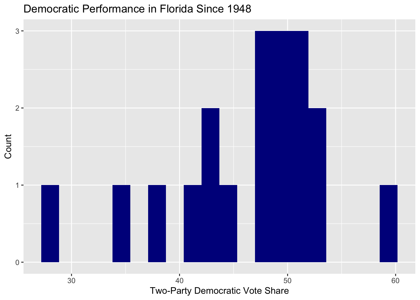
(a) Histogram

In ggplot, plot a histogram of the two-party Democratic vote share in Florida going back to 1948 with geom_histogram. Label the chart as appropriate and play with different numbers of bins and theme settings until you have a chart style you are satisfied with.

florida_hist <- ggplot(combined_data_wide, 
       mapping = aes(x = Democrat_Florida)) +
  geom_histogram(bins = 20, fill = "darkblue") +
  xlab("Two-Party Democratic Vote Share") +
  ylab("Count") +
  ggtitle("Democratic Performance in Florida Since 1948")
florida_hist

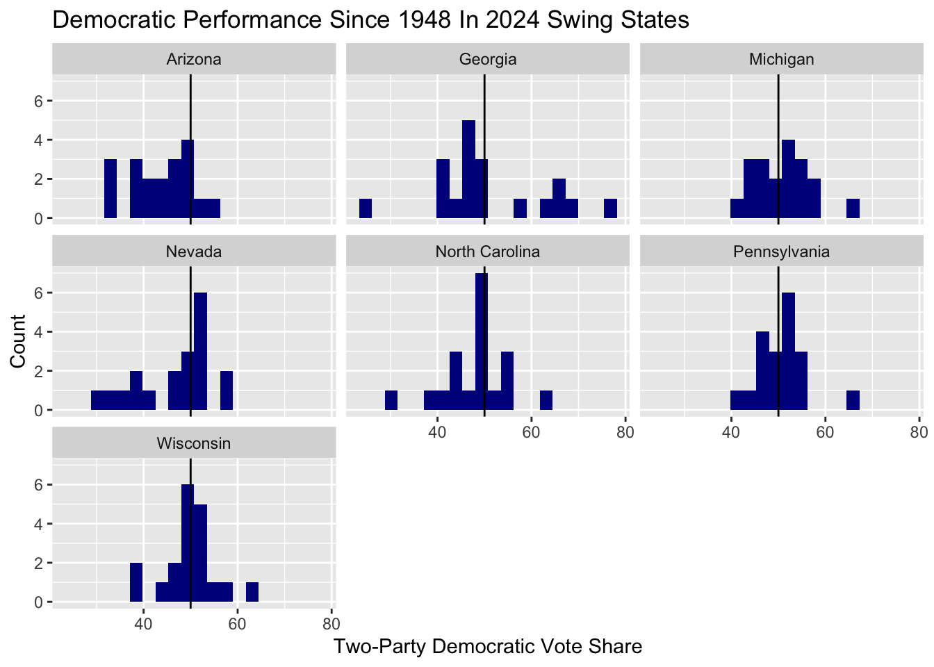
dem_swing <- combined_data |>
  filter(party == "Democrat") |>
  filter(state == "Georgia" | state == "Michigan" | state == "Arizona" |
           state == "Wisconsin" | state == "Nevada" | state == "Pennsylvania" |
           state == "North Carolina")

state_hist <- ggplot(data = dem_swing, 
                     mapping = aes(x = two_party_vote_share)) +
  geom_histogram(bins = 20, fill = "darkblue") +
  facet_wrap(~ state) +
  xlab("Two-Party Democratic Vote Share") +
  ylab("Count") +
  ggtitle("Democratic Performance Since 1948 In 2024 Swing States") +
  geom_vline(xintercept = 50)
state_hist

(b) Scatterplot

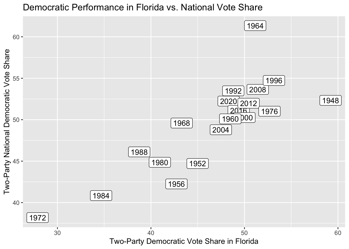
In ggplot, plot a scatterplot of the two-party Democratic vote share in Florida going back to 1948 on the x-axis and the national Democratic two-party vote share on the y-axis. Instead of dots, label each point with the election year using geom_label. Also label the chart as appropriate and play with different theme settings until you have a chart style you are satisfied with.

florida_scatter <- ggplot(combined_data_wide, 
                          mapping = aes(x = Democrat_Florida, y = dem_tpv,
                                        label = year)) +
  geom_label() +
  xlab("Two-Party Democratic Vote Share in Florida") +
  ylab("Two-Party National Democratic Vote Share") +
  ggtitle("Democratic Performance in Florida vs. National Vote Share")
florida_scatter